Introduction

During embryogenesis, cells repeatedly divide and dynamically change their position in 3D space, resulting in a highly dynamic environment. A number of studies have tried to acquire quantitative criteria such as chromosome numbers, the synchrony of cell division, and the rate of development, using image segmentation.

However, the existing solutions have abritrarily-determined hyperparameters, and low segmentation accuracy due to suboptimal analysis of spatiotemporal variations in the time-series data. With regard to fluorescence microscopic imaging, a time series of $\mathbb R^3$ images analysis is difficult as the fluorescence intensity decreases along the z-axis, because the innermost part of the embryo is not fully transparent. Furthermore, fluorophore fading causes decreasing fluorescence intensity with time.

Tokuoka et al.¹ propose QCANet to generalise and improve segmentation accuracy of 3D fluorescence microscopic images. They show that by decomposing the task into separate convolutional neural networks (CNNs) responsible for semantic and instance segmentation, they can outperform the 3D U-Net baseline². In this post, we try to replicate their results and highlight discrepancies in our reproduction.

Background

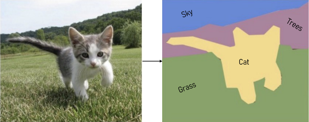
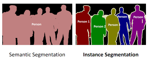
In the world of image processing, semantic segmentation refers to labelling each voxel in an image with the correct class. E.g. in , the cat, trees, sky and ground are shown. Whereas instance segmentation partitions this class into distinct instances. E.g. divides a group of people into individuals.

Semantic Segmentation

Instance and Semantic Segmentation

Instance and Semantic Segmentation

Approach

QCANet Architecture

As shown in , QCANet consists of two subnetworks: Nuclear Segmentation Network (NSN), and Nuclear Detection Network (NDN); responsible for semantic segmentation and instance segmentation. These two networks operate on the input individually, as seen in [fig:segmentation-pipeline], and their outputs are then combined in the post processing phase.

Segmentation Pipeline

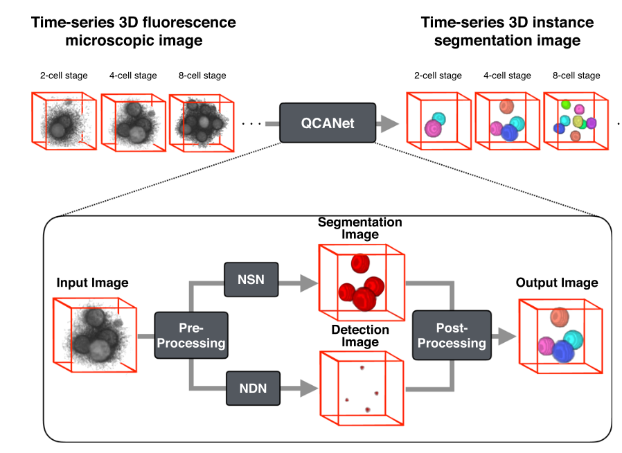
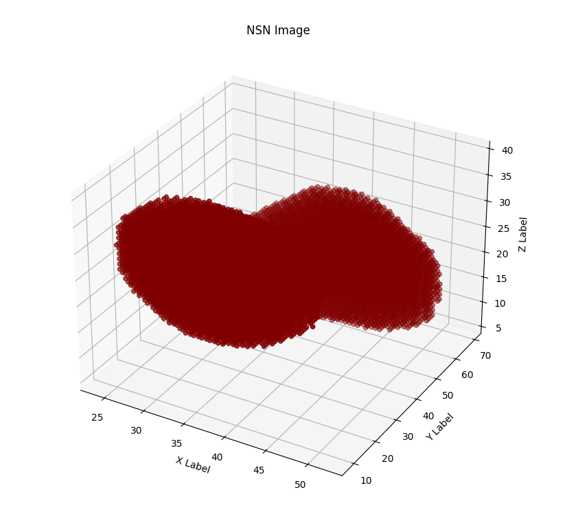
The primary objective of the NSN is to segment the nuclear regions (from the background) in the images. In other words, it must detect all voxels in the 3D image belonging to nuclei. This network outputs a binary mask which covers all the detected nuclei in the 3D image by using a series of 3D convolutional layers, max pooling layers aswell as deconvolution and concatenation (an output from a previous downsampling layer is concatenated with the output at the current, upsampled layer to ensure that enough information is present when upscaling by adding back features found in previous layers) layers based on the 3D U-NET architecture . The final layer is then passed through a softmax function to convert the numerical output into values between 0 and 1 denoting the probability that the specific voxel represents part of a nucleus.

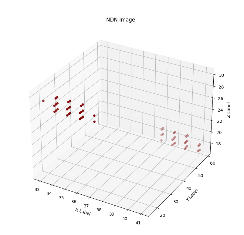
The NDN, on the other hand, learns to fully mask an image except for the nuclear centres. This, when combined with the output of the NSN allows the QCANet to perform instance segmentation on individual nuclei. As with the NSN the architecture is based on the UNET-3D architecture and, although many more layers are used, they can once again be broken down into convolutional, max pooling, deconvolution and concatenation layers. As in the NSN, the output is passed through a softmax function.

Pre-Processing

As we are reproducing the authors’ works and aim to achieve similar results, we emulated their exact pre-processing steps, which consist of interpolation and mirror padding. First, we interpolate the given images in the dataset. Depending on the microscopy approach and manufacturer, 3D images do not usually come in the form of a 1:1:1 ratio. In most cases, interpolation is needed to account for higher z dimension ratios. Another pre-processing step we perform is padding, which is done to ensure that all images are of the same size. As the background around the edges is slightly noisy and does not consist of strictly zero values, mirror padding seems to be most appropriate to end up with a consistent processed image. The QCANet authors further implement data augmentation by flipping each image along its x and y dimensions, to address their small training set size.

While data augmentation quadruples the training set size, it also makes training take four times as long. Given the limited amount of time to reproduce the project, and the extra training time overhead that data augmentation added, we decided against following this pre-processing step.

Post-Processing

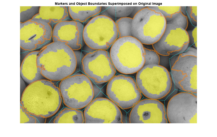
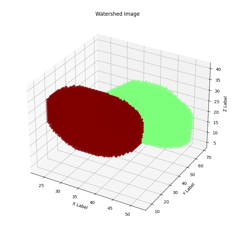
When the outputs of the the NSN and NDN are found, they need to be combined. To complete QCANet’s cell-instance segmentation, marker-based watershed divides the semantic segmentation region with the identified centres as markers. An illustrative example of this process is shown in [fig:watershed]. Watershed ‘floods’ the central markers to accurately separate each nucleus; which helps in preventing over-segmentation as the flood is less likely to be affected by noise or artifacts.

Marker Based Water Shed

Experiment Setup

3D Cell Dataset

The dataset consists of a series of frames, each one of them being a 3D image of cells. The entire series of frames, when appended and watched as a short film, shows the cells’ movements and their process of splitting. The authors manually labelled a ground truth for the training set at 11 time points in 11 mouse embryos.

Although our network was trained on this specific dataset, inference can be done on all datasets with similar 3D images of cells. However, our current codebase was only tested on tiff files, which are made of 2D frames that are stacked on top of each other to create a 3D image.

Training Dice Loss

Both the NSN and NDN use dice loss. The Dice loss is a common loss function for image segmentation which measures the overlap between the predicted and target masks. In addition, the dice loss also solves another important problem: the unbalance between the labels (the number of pixels or voxels in the background and objects). In the segmentation task, it is often a problem that labels (the number of pixels or voxels in the background and objects) are not balanced; the use of dice loss function as an objective function can suppress the influence of dataset label imbalance.

For boolean data (0 or 1) the equation is as follows:

$$DL = 1- DC = 1 - \frac{2 \cdot TP}{|y| + |\hat{y}|}$$

NSN and NDN Hyperparameters

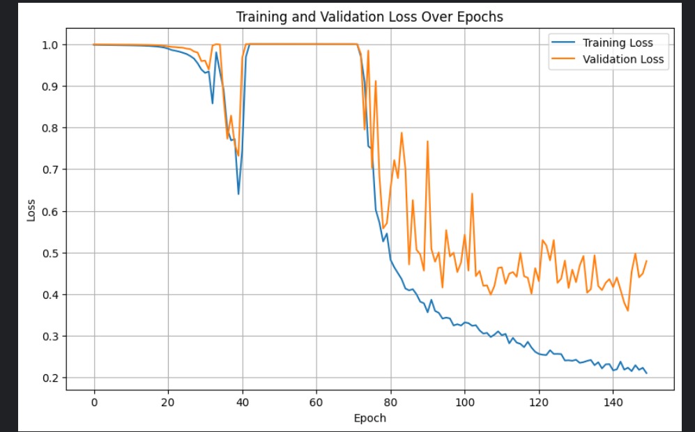
The hyperparameters and optimization algorithm used for both networks can be found in [tab:hyper_summary]. It must be noted that the learning rate for the NSN was increased compared to the paper as when using the learning rate described in the paper the loss would not decrease while training.

	NSN	NDN
Optimizer	SGD	SGD
Learning rate	0.1	0.1
Batch Size	4	4
num Epochs	80	150

The hyperparameters used to train each model

Evaluation Metrics

The intersection of Union (IoU) is a metric which measures the overlap between bounding boxes: one from the network and one the ground truth. Conventionally this is used to measure false positive (FP) or false negative (FN) rates, however it cannot identify instance segmentation as it looks at all the cells.

$$IoU = \frac{TP}{TP + FP + FN}$$

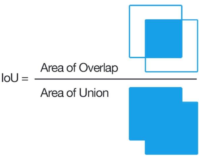
Semantic Evaluation using Geodesic distances or SEG reviews the accuracy of the image segmentation, as in how closely the segmentation from the network matches that of the ground truth segmentation. Below is the mathematical notation for SEG, in essence it is the sum over all ground truths, where for each one the maximum IoU is computed with respect to the prediction of the network, before being normalised by the total number of predictions. Here it evaluates the absence of FNs.

$$SEG = \sum_{j}^{N_i} \frac{1}{N_i} \max_i IoU(y_i, y_j^*)$$

The Mean Unweighted Coverage (MUCov), is alike to SEG however in the perspective of the predicted output, as shown below. Here, it evaluates the absence of FPs.

$$MUCov = \sum_{i}^{N_j} \frac{1}{N_j} \max_j IoU(y_i, y_j^*)$$

Results

Learning curves

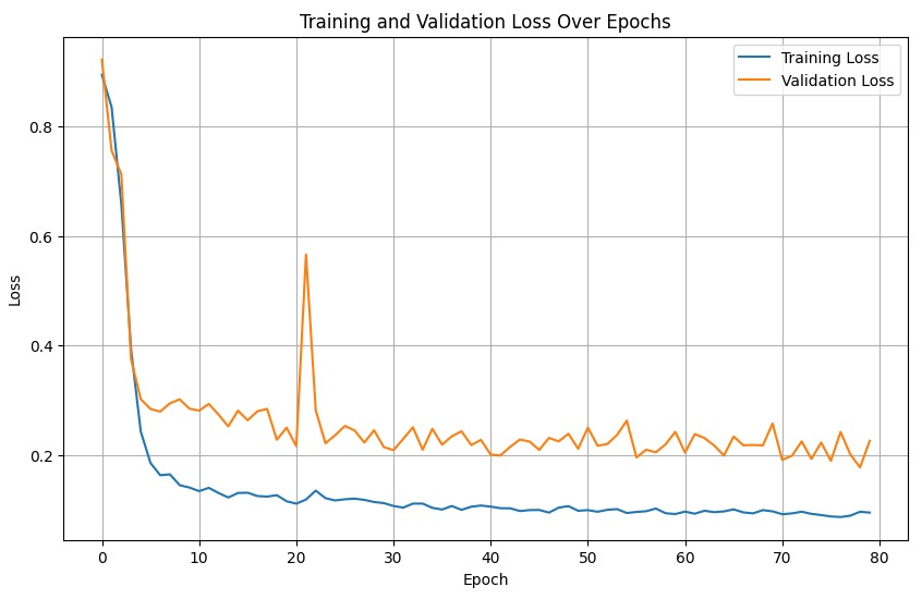
The two figures below show the learning curves for the NSN and the NDN training and validation loss per epoch, respectively.

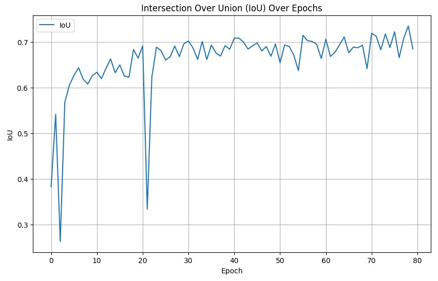
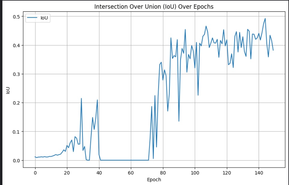
And below are the IoU scores over epochs for the NSN and NDN networks, respestively.

Quantitative results compared to the original paper

After training our two networks and implementing the post-processing steps, it was time to evaluate is against the original paper. For the three previously mentioned metrics, we ran inference on our version of the QCANet, over all images in the test set. The results, as compared to the original QCANet, can be seen in .

	IoU	SEG	MuCov
Original QCANet	0.746	0.710	0.721
Our implementation	0.503	0.155	0.079

Our network run and evaluated on three segmentation metrics vs. the results of the original paper

Evidently, our results are far worse than those cited in the paper, specifically for the SEG and MuCov metrics. Since the IoU for our implementation is quite good and it is a semantic segmentation metric, it is clear that the NDN is the component that is lacking. We discuss the quantitative discrepancy further in .

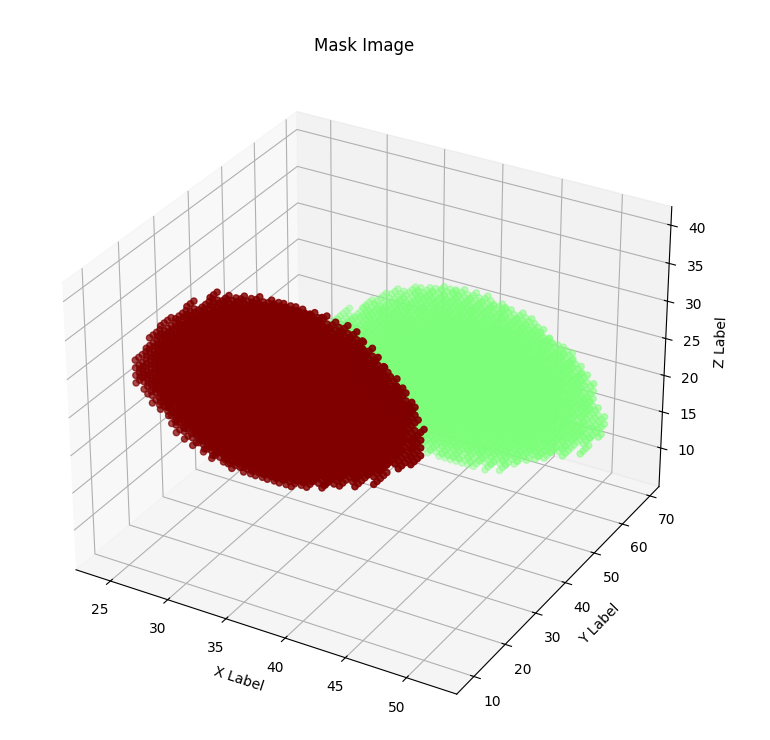
Although we achieved much worse quantitative results than the original paper, we are quite happy with the way the output images look, in a visual sense. Here is an example of the pipeline running with all intermediate images, for an image in the test set:

Discussion

Limitations

Although the QCAnet was correclty implemented, in the sense that we can now perform satisfactory instance segmentation on 3D images of cells, the quantitative results we achieved are not very close to the paper and lack to varying degrees in all three metrics.

Implementing the NSN and the NDN were not daunting tasks, and we were able to get the architectures correct within a few hours. The most time consuming task was training, which required us to tweak parameters multiple times, run multiple training runs that stop early, and experiment until we got satisfactory training curves. Ironically, Tokuoka et al. claimed QCANet would relieve this heuristic, application-dependent hyperparameter search.

Given that we had limited time and limited Kaggle credits to train, we did not implement data augmentation, which would have quadrupled the number of training instances in our dataset and most likely led to even better results. This is most likely the biggest gap between our implementation and the paper’s implementation. Further inconsistencies that we took in order to get a working result instead of a very precise one, are discussed in the following section.

Reproducibility Assessment

Although the paper tried to be detailed and precise with regards to their approach, there are many changes we had to make to achieve acceptable results. Many of their choices are not well motivated, and reproducing their entire instance segmentation pipeline requires a lot of trial and error.

For researchers trying to reproduce the approach proposed by the paper, we suggest that they do not worry about the exact hyperparameters and architectures they use. Instead, focus just on having two working semantic segmentation networks - one for the cells and one for the cell centers. The method of combining the output of two semantic segmentation networks using marker-based watershed to perform instance segmentation on 3D cells is indeed valid and it works well, but the hyperparameter choice should be left to the person implementing and not copied from the paper.

Leaving the choice of hyperparameters and architectures to the person reproducing the method is especially important in the case of the NDN. Here, the paper proposes a huge network that has too many steps in the down (convolutional and max pool) direction and in the upwards (convolution and upsample) directions. NDN has millions of extra parameters than the standard 3D U-NET and it is likely that not all are necessary. If the goal were to reproduce the approach to an acceptable level and not the results specifically, we recommend a standard 3D U-NET for the NDN.

The paper also uses strange hyperparameters that are not well motivated, like a kernel size of 5 for the NDN which is not standard. The architecture mentioned uses kernel sizes of 5, a padding of 1 and a stride of 1 for each upsampling step. However, such a combination of kernel sizes, padding and stride downsamples the input by 1 pixel on each side after each step. In order to remedy this, the last convolutional layer should have a padding of 4, but the paper shows a padding of 0 for that layer. The architecture of the NDN is therefore not even consistent, and we were left with the choice between changing the kernel size to 3 or adding a padding of 4 to the last layer. In the end, we changed the kernel size of each convolutional layer in the NDN to 3.

Here is the full list of hyperparameters we had to specify differently in order to get acceptable instance segmentation results:

• Optimizer: the paper proposed Adam as an optimizer for the NDN, which can be more stable than SGD thanks to the momentum and RMSprop mechanisms. We used SGD for the NDN, which was the only optimizer where the IoU was able to increase. This is most likely because the search space of the NDN - given its number of parameters - is massive, and the high variance that SGD suffers can actually be an advantage in this case.

• Learning rate: Instead of 0.01, we actually used a very high learning rate of 0.1. It seems as though the search space is very flat, and a lot of iterations are needed to reach areas of high gradients. A learning rate of 0.1 sped up the process of reaching points where the dice loss would decrease, at a certain IoU it was decreased to 0.02.

• NDN architecture: as previously mentioned, the NDN was modified to have a kernel size of 3 instead of a kernel size of 5.

• Data augmentation: unlike the paper, we perform no data augmentation because it makes the process of training too time consuming given the amount of time and Kaggle credits we had to train our models.

• Number of epochs: the NSN was starting to overfit very easily after 60 or so epochs, and the test accuracy was not decreasing. We therefore opted for 80 epochs instead of 150.

As for comparing the results of the QCAnet with current state-of-the-arts methods in instance segmentation, only Mask-RCNN can be used in a fair comparison using the metrics stated. The paper unfairly compares their approach to the traditional 3D U-NET, which is designed for semantic segmentation and not instance segmentation.

Conclusion

The authors of QCAnet propose a great novel approach to instance segmentation that combines two semantic segmentation networks and post-processing in the form of marker-based watershed, and we were able to reproduce the method successfully. However, a lot of choices had to be made by us instead of blindly following the choices of the authors, and an exact reproduction is therefore not very easy to achieve.

References

1. Y. Tokuoka et al., ‘3D convolutional neural networks-based segmentation to acquire quantitative criteria of the nucleus during mouse embryogenesis’, npj Syst Biol Appl, vol. 6, no. 1, p. 32, Oct. 2020, doi: 10.1038/s41540-020-00152-8. ↩

2. Ö. Çiçek, A. Abdulkadir, S. S. Lienkamp, T. Brox, and O. Ronneberger, ‘3D U-Net: Learning Dense Volumetric Segmentation from Sparse Annotation’. arXiv, Jun. 21, 2016. Accessed: Apr. 10, 2024. [Online]. Available: http://arxiv.org/abs/1606.06650 ↩